A system design begins with the workload and constraints, not with a cloud product. Capacity estimation translates business requirements into rates, storage, memory, network bandwidth and failure budgets. An estimate is a scenario based on assumptions, not a prediction; document its units and sensitivity [1].
Workload definitions#
- Request rate: average requests per second (RPS) equals requests per day divided by 86,400 seconds, assuming an even mean over a day.
- Peak-to-average ratio: an assumption such as 8×, which must be measured or treated as hypothetical.
- Concurrency: number of overlapping requests, not number of registered accounts.
- Throughput: completed operations or transferred bytes per second.
- Latency: elapsed time per operation, reported as a distribution including p95/p99 rather than only an average.
Little's law, under stable conditions with consistent observation boundaries, relates average in-system requests L, throughput λ, and average time W: L=λW. Thus at 100 RPS and average 0.2 seconds, average concurrency is about 20. This does not imply that only 20 requests can overlap during a burst, nor does it predict tail latency near saturation.
Worked scenario with explicit assumptions#
Assume a read-heavy service receives 12 million requests/day; 95% reads; peak load is eight times the average; each response transfers 3 KiB; one application instance sustains 400 RPS at a tested safe utilization; and deployed capacity must survive one instance failing.
| Quantity | Calculation | Estimate |
|---|---|---|
| Mean total RPS | 12,000,000 / 86,400 |
139 RPS |
| Peak total RPS | 139 × 8 |
1,112 RPS |
| Peak read RPS | 1,112 × 0.95 |
1,056 RPS |
| Peak outbound payload | 1,112 × 3 KiB |
~3.26 MiB/s |
| Instances required at peak | ceil(1,112 / 400) |
3 |
| Provisioned for one failure | 3 + 1 |
4, assuming traffic rebalances |
The 400 RPS limit must come from benchmarking with the intended request mix and downstream dependencies. Choosing a bigger machine does not automatically remove a serialized database bottleneck. Raw payload estimates exclude headers, TLS overhead, retransmissions and replication.
Estimate storage separately#
Suppose 20,000 new records arrive daily, average payload 2 KiB. Raw payload growth is roughly 40,000 KiB/day, about 14 GiB/year before indexes, replicas, logs, compression and backup copies. Define retention requirements first; multiplying only by the data replication factor still misses operational overhead.
Distinguish logical size from provisioned physical disk and mean throughput from burst capacity. Store measured assumptions alongside the design and revise them after load tests. A design that cannot state its assumptions cannot be falsified.
Saturation and resilience#
As utilization approaches a constrained resource's limit, queuing delay can increase sharply, even when average request volume remains unchanged. Protect the system with bounded queues, admission control, timeouts, circuit breakers and explicit overload behavior. Availability and latency must be expressed through measurable service-level indicators and objectives (SLIs/SLOs) [1][2].
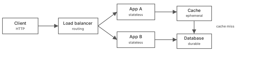
The diagram is a possible read path, not an instruction to add every component. A small application may correctly start with a single service and relational database.
A capacity model must have units and a saturation curve#
The arithmetic instances=ceil(peak_RPS / tested_RPS_per_instance) is meaningful only when the denominator is measured at the required latency and error budget. A benchmark reporting the maximum throughput at 100% CPU cannot be used as a safe per-instance operating target. Load depends on request mix, payload size, data locality, connection reuse, background jobs and downstream saturation. For each assumption, record a plausible range and rerun the estimate with pessimistic values [1].
Separate arrival rate λ (jobs/s), service rate μ (jobs/s per worker) and concurrency L (jobs in system). Little's law L=λW holds for stable systems over consistent observation boundaries; it does not by itself predict response-time distribution. For a single idealized M/M/1 queue with Poisson arrivals and exponential service times, mean time in the system is W=1/(μ−λ) when λ<μ; this is a model, not a universal production formula. As λ approaches μ, delay diverges. Real services with bursty arrivals or multiple resource constraints can behave differently.
Redundancy and failure budgets#
Suppose peak traffic is 2,400 RPS, and a server sustains 600 RPS at the desired latency under the intended mix. To target 60% of that tested ceiling, plan 600×0.60=360 RPS per node. ceil(2400/360)=7 healthy nodes cover the modeled peak. To survive one node failing while keeping the same target, provision 8. This is a scenario: if the database cannot supply 2,400 RPS, adding replicas to the application tier will not make the end-to-end service scale.
A 99.9% monthly availability SLO corresponds to approximately 43.2 minutes of total allowed unavailability over a 30-day month, if measured as a simple time proportion. But a request-based SLO may count failed requests rather than minutes, so converting directly to a time budget may be misleading [2]. Clearly define the measurement and error criteria.
Storage, bandwidth and retention#
For N new records/day, mean logical record size S bytes and retention D days, raw live logical storage is N×S×D, ignoring deletion and compression. Physical demand adds indexes, replication, transaction logs, backup retention, filesystem overhead and headroom. For network transfer, distinguish decimal MB from binary MiB and whether you are counting payload, wire bytes or compressed transfer. Read-heavy systems may be bandwidth-constrained long before CPU saturation.
| Unknown | Experiment to reduce uncertainty |
|---|---|
| Peak-to-average ratio | Measure traffic by time bucket, region and endpoint |
| Per-instance capacity | Load test against representative downstreams |
| Cache hit fraction | Compare warmed and cold cache windows |
| Traffic mix | Break down cost by endpoint and user tier |
| Recovery margin | Kill one replica during load and inspect p99 |
Test design and decision record#
Run a steady-state test, a burst test, a cold-start test and a failure-over test. Each should specify offered load, completed throughput, p95/p99, errors, CPU, memory, queue depth and downstream health. If offered load increases while successful throughput stops growing, the difference must be rejected or accumulate as backlog; simply counting accepted requests hides overload. Document the point where admission control becomes necessary [1].
Checkpoint: if one replica fails, estimate capacity using remaining replicas. If you use a cache hit rate of 95%, quantify the origin load when that hit rate suddenly becomes 0%; resilience depends on the surge, not only normal operation.
Exercises and verification#
- If average traffic doubles but peak ratio stays constant, redo instance provisioning while preserving one-failure tolerance.
- At 500 RPS and average response time 0.4 seconds, Little's law suggests mean concurrency
200in a stable system. Explain why p99 latency may still be much higher. - List at least three real measurements needed before committing to a cost estimate: request distribution, payload size, service capacity under load and database query distribution are examples.
Good estimates are orders-of-magnitude tools that drive conversations about trade-offs; they should not be presented as precise capacity guarantees.