SQL describes what rows a query must produce; the database planner chooses a physical strategy for producing them. Equivalent relational results can arise from very different access paths, join orders and intermediate result sizes. SQL performance is therefore not reducible to whether a query contains an index or whether its text is short. A correct diagnosis separates logical semantics from estimated execution cost and observed runtime [1].
From relational operations to physical operators#
A SELECT statement may require filtering (selection), column projection, join, grouping and ordering. A planner can rearrange many operations when semantics permit, pushing filters earlier or changing join order. A physical plan then chooses operators such as sequential scan, index scan, hash join, merge join, nested loop and sort. The same SQL statement can produce a different plan when table size, statistics or parameters change.
An optimizer's cost is generally an internal relative estimate, not elapsed milliseconds. Comparing estimated costs can help select among candidate plans, but treating an EXPLAIN cost of 100 as 100 ms is a category error. The optimizer uses assumptions about disk and CPU cost, data distribution and estimated cardinalities [1][2].
Selectivity and cardinality estimates#
Let N be input rows, s the proportion satisfying a predicate. Expected matching rows are roughly N×s when s is a sensible estimated selectivity. For independent predicates A and B, one might approximate joint selectivity as s_A×s_B. But correlation breaks this assumption. Suppose a 10,000-row dataset contains 1,000 Brazilian customers, and all 1,000 use a specific regional payment setting. Each individual predicate matches 10%; independence predicts 10,000×0.1×0.1=100 matches, whereas the actual conjunction returns 1,000. This tenfold underestimation can cause an unsuitable join or scan [2].
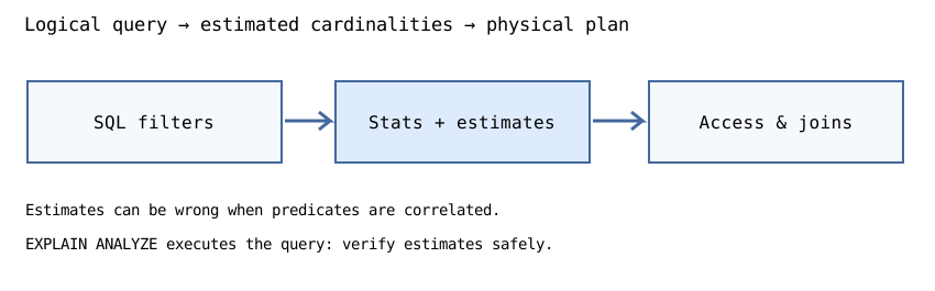
PostgreSQL collects distribution statistics, including frequent values and histograms, through ANALYZE; statistics are based on samples and can be inaccurate, especially for skewed or correlated columns [4]. Extended statistics can represent multivariate relationships where single-column assumptions fail [2]. Increasing the statistics target trades planning information quality against sampling and catalog overhead; it does not guarantee perfect plans.
Composite index ordering#
A B-tree on (tenant_id, created_at) groups index entries primarily by tenant and secondarily by creation time. An equality filter on tenant plus range filter on created_at can efficiently constrain an ordered region. A filter only on created_at often has a weaker access path because the leading key is unconstrained. Modern PostgreSQL also has skip scan optimizations in some conditions, so the simplistic statement 'an index can never be used without its first column' is false [3].
Multiple single-column indexes and one composite index are not equivalent. A composite key can preserve an ordering useful for a query; individual indexes may instead require bitmap combination and extra heap work. Adding indexes is not free: writes, vacuum and storage overhead increase. Design indexes from measured high-value queries and verify the planner's behavior.
Join strategies and their assumptions#
A nested-loop join scans the inner input for each outer row, or can probe an index efficiently when the outer side is small and the inner key is indexed. A hash join builds a hash table on one input and probes it with the other, often fitting equality joins when memory and key semantics allow. A merge join benefits from sorted inputs and can be attractive when the data is already ordered or sorting is justified. The planner estimates intermediate cardinality because a badly ordered large join may materialize far more rows than expected [1].
| Strategy | Strength | Failure mode |
|---|---|---|
| Nested loop + indexed inner | Tiny outer input and selective probes | Excessive repeated probes if outer grows |
| Hash join | Equality join on sizeable relations | Hash build spills under memory pressure |
| Merge join | Already sorted inputs | Sorting cost dominates if order absent |
| Sequential scan | Large fraction of table | Wasteful for highly selective predicates |
| Index scan | Selective access | Random heap fetches on many rows |
Choosing a join type by habit without knowing row counts is not engineering reasoning. Neither is forcing index scans simply because a B-tree exists: if most table pages must be visited, a sequential strategy may be faster.
Read EXPLAIN and verify predictions#
Plain EXPLAIN displays a chosen plan and estimated costs and rows without executing the query. EXPLAIN ANALYZE actually executes the statement and reports observed times and row counts. Therefore wrapping INSERT, UPDATE or DELETE in EXPLAIN ANALYZE can change real data; use explicit transaction rollback or a safe test environment when examining writes. Compare estimates with actual rows and loops, not only total milliseconds. Check buffers and I/O to understand whether the work reads cached pages or storage [1].
A common red flag is estimated rows=10 but actual rows=100,000 at an early node. The optimizer may select nested loops expecting tiny intermediate results. Another concern is a plan with inexpensive startup time but very large total work; LIMIT, ORDER BY and cursor use can change what actually matters. Explain numbers are contextual; repeat measurements under representative data and cache states.
Executable cardinality reasoning#
def independent_estimate(rows, *selectivities):
    if rows < 0 or any(not 0 <= s <= 1 for s in selectivities):
        raise ValueError("invalid row count or selectivity")
    result = rows
    for s in selectivities:
        result *= s
    return round(result)

assert independent_estimate(10000, 0.1) == 1000
assert independent_estimate(10000, 0.1, 0.1) == 100
actual_correlated = 1000
assert actual_correlated / independent_estimate(10000, 0.1, 0.1) == 10
The function models an independence assumption, not the PostgreSQL optimizer or a statistical confidence bound. The actual count comes from the stated hypothetical data distribution; it is not measured from a live database. For a real query, capture row-count estimates and measurements with EXPLAIN and the environment's data distribution.
Operational counterexamples#
A predicate written with an implicit type conversion can prevent an intended access path or change selectivity estimates. A correlated predicate can invalidate per-column independence. A poorly chosen ORDER BY can force a large sort. A LIMIT may encourage early-stop plans that perform poorly if the requested rows are rare. Timeouts or blocked transactions can dominate latency even when CPU execution and plan choice are efficient.
Avoid interpreting one warm-cache benchmark as a robust performance guarantee. Query plans can change after ANALYZE, schema migrations and large shifts in data skew. The correct feedback loop is hypothesis → plan inspection → representative measurement → carefully scoped index/query change → regression verification.
Prerequisite connections: Database pages and WAL explain physical tuples and index pointers; complexity analysis distinguishes cost models from empirical time; caching discusses how warm data changes actual latency.
Exercises and verification#
- For N=50,000 and independent predicates with selectivities 0.2 and 0.05, estimate 500 rows. Explain why correlation can invalidate the answer.
- Describe when a composite (tenant, created_at) index helps and when it may be less useful than an alternative.
- State the difference between EXPLAIN and EXPLAIN ANALYZE, including the risk with data-modifying queries.
- Explain a scenario in which a sequential scan is preferable to an available B-tree index.
- Given estimated join input 100 rows versus actual 1,000,000, describe why nested-loop probing could become unexpectedly expensive and which evidence to collect.