Sorting rearranges values into an ordering established by a comparator or key. That sounds simple, but algorithms vary in guarantees about input order, stability, time, extra memory and whether data can be modified in place. An engineer should select a sorting method by its contract, not only by memorizing that O(n log n) is good. General-purpose Python sorting is stable and highly optimized, so implementing sorting from scratch is primarily useful for algorithmic reasoning, custom constraints and understanding the trade-offs [3].
Ordering, stability and comparator contracts#
For values a[0..n−1], a nondecreasing ordering satisfies a[i]≤a[i+1] for each valid adjacent index. A stable sort also preserves the original relative order of records whose sort keys compare equal. If two messages share priority 4 and entered as A then B, a stable sort by priority places A before B. It does not guarantee order among distinct priority keys, and stability is not a guarantee of preserving original indices under arbitrary comparators.
Comparisons must define an ordering suitable for sorting, normally transitive and consistent. A comparator that alternates answers or depends on mutable global state can invalidate proofs. Likewise, NaN behaves unusually under floating comparisons, so decide an explicit policy when total ordering is required. Duplicates, empty sequences, already-sorted and reverse-sorted input all belong in the test set.
Insertion sort: invariant and quadratic cost#
Insertion sort scans from left to right maintaining the prefix [0,i) in sorted order. For each next element, shift larger prefix elements to the right and insert the new value in its ordered position. The invariant is: before processing index i, all previous i elements are sorted and are a permutation of the first i original elements. The insertion preserves ordering and the multiset of values. By induction, the entire array is sorted at termination.
Insertion sort's best case is Θ(n) comparisons on an already ordered input with an early-stop inner loop. Its worst-case time is Θ(n²), such as reverse order: the shifts sum 1+2+...+(n−1). It uses O(1) extra storage in its normal in-place form and is stable if equal elements are not moved past each other. This makes it useful for small arrays and almost-sorted runs, not large arbitrary datasets.
Mergesort: independent halves and a stable merge#
Mergesort splits the range in two, sorts each half recursively, then merges the sorted halves. To merge, keep two read indices; append the smaller next key to an output buffer, advancing only that index. The invariant is that the output is sorted and contains precisely the smallest already-consumed items from the two halves. When equal keys are encountered, choosing the left item first preserves their original cross-half order [1].
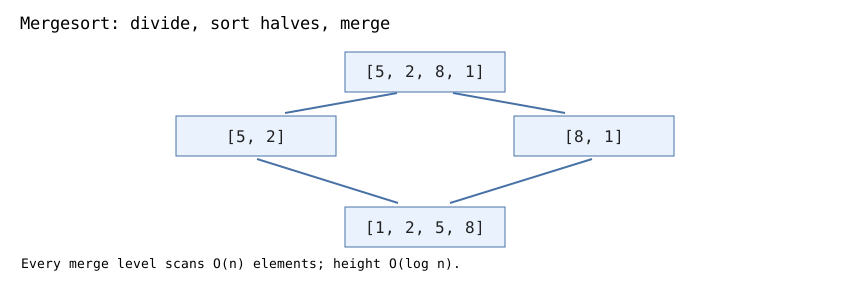
The following implementation accepts records with a key supplied by a function. It creates new lists and leaves the input unchanged. The key function should be deterministic and its resulting values comparable.
def stable_mergesort(items, key=lambda x: x):
    if len(items) <= 1:
        return list(items)
    midpoint = len(items) // 2
    left = stable_mergesort(items[:midpoint], key)
    right = stable_mergesort(items[midpoint:], key)
    merged = []
    i = j = 0
    while i < len(left) and j < len(right):
        if key(left[i]) <= key(right[j]):
            merged.append(left[i])
            i += 1
        else:
            merged.append(right[j])
            j += 1
    merged.extend(left[i:])
    merged.extend(right[j:])
    return merged

values = [(2, "A"), (1, "B"), (2, "C"), (1, "D")]
assert stable_mergesort(values, key=lambda r: r[0]) == [
    (1, "B"), (1, "D"), (2, "A"), (2, "C")
]
assert values[0] == (2, "A")
assert stable_mergesort([]) == []
assert stable_mergesort([9]) == [9]
assert stable_mergesort([5, -1, 5, 0]) == [-1, 0, 5, 5]
Merging k elements costs Θ(k) because each item is appended once. The recurrence T(n)=2T(n/2)+Θ(n) therefore solves to Θ(n log n), assuming constant-time key comparison. Recursion depth is O(log n). Because slices and merged lists allocate storage, this particular Python implementation may use extra temporary allocations across recursion; peak simultaneously reachable element storage remains O(n) for this balanced implementation, plus O(log n) call frames. The algorithm is not in-place.
Quicksort: partition invariant and its worst case#
Quicksort selects a pivot, partitions the array into elements less than and greater than or equal to that pivot under a consistent partition scheme, then sorts the partitions. A common in-place Lomuto partition maintains an interval [lo,k) of elements known to be ≤pivot, with the scanned part separating known large elements from not-yet-inspected ones. After placing the pivot at its final index, both recursive subranges are smaller [2].
Balanced partitions lead to recurrence T(n)=2T(n/2)+Θ(n), yielding Θ(n log n). But choosing the last element as pivot on already sorted input can repeatedly produce ranges of sizes n−1 and 0, so T(n)=T(n−1)+Θ(n)=Θ(n²). Randomizing the pivot gives expected Θ(n log n) comparisons under the usual randomized assumptions, not a deterministic worst-case guarantee. Typical in-place quicksort is not stable without extra machinery; its recursion depth can reach Θ(n) under unbalanced partitions.
Duplicate-heavy inputs deserve a three-way partition that groups values smaller than, equal to and greater than the pivot. This can avoid unnecessary repeated partitioning of many equal keys. The same idea also appears in quickselect, which seeks an order statistic rather than sorting the whole array.
Heapsort: a heap invariant without extra merge buffer#
A max-heap keeps each parent at least as large as both children. Store a complete binary tree in an array: children of index i are 2i+1 and 2i+2. Build a max-heap in O(n) time by sifting down internal nodes from the bottom upward; then swap its maximum at index 0 with the end of the active prefix and restore the heap over the shorter prefix. The invariant is: the active prefix is a max-heap and the suffix already contains the largest elements in ascending final order.
def heapsort(items):
    a = list(items)
    n = len(a)
    def sift_down(root, end):
        while True:
            child = 2 * root + 1
            if child >= end:
                return
            if child + 1 < end and a[child] < a[child + 1]:
                child += 1
            if a[root] >= a[child]:
                return
            a[root], a[child] = a[child], a[root]
            root = child
    for i in range(n // 2 - 1, -1, -1):
        sift_down(i, n)
    for end in range(n - 1, 0, -1):
        a[0], a[end] = a[end], a[0]
        sift_down(0, end)
    return a

cases = [[], [1], [3,1,2], [2,2,2], [9,-1,4,0,9], list(range(10)), list(range(9,-1,-1))]
for case in cases:
    assert heapsort(case) == sorted(case)
Heap construction runs in Θ(n) time: most nodes are near leaves and require little sifting. Each of at most n removals of the current maximum performs O(log n) work, so worst-case total sorting time is O(n log n). The implementation copies its input and thus uses O(n) space for the returned list; the core heap operations, once a list is available, need O(1) auxiliary space. Standard heapsort is not stable [1].
Comparison table: guarantees versus favorable inputs#
| Method | Worst-case time | Extra space (usual form) | Stable? |
|---|---|---|---|
| Insertion sort | Θ(n²) | O(1) | Yes if equals stay ordered |
| Mergesort | Θ(n log n) | O(n) buffer | Yes with left-first ties |
| Quicksort | Θ(n²) | O(log n) expected call stack, Θ(n) worst | Typically no |
| Heapsort | O(n log n) | O(1) when in-place | Typically no |
| Python sort / sorted | O(n log n) worst-case comparisons in the documented Timsort family | Implementation-dependent | Yes [3] |
Do not confuse in-place with stable, or expected with worst-case bounds. Worst-case Θ(n log n) for comparison sorts is asymptotically optimal: there are n! permutations of n distinct keys, and a binary comparison decision tree needs at least log₂(n!)=Ω(n log n) comparisons in its worst branch. Counting/radix sorts can beat that bound when keys have exploitable structure and non-comparison operations are permitted.
Choose algorithms for a concrete workload#
For small nearly sorted runs, insertion sort is straightforward and may be fast. To guarantee stable order among duplicate business keys, use stable sort or attach original indices as explicit secondary keys. For a memory-constrained environment that demands worst-case O(n log n) comparisons, in-place heapsort can be attractive. For large Python application lists, use the language's standard sorting facility rather than a toy Python mergesort or heap sort unless a measurable requirement justifies it [3].
Exercises and verification#
- Trace insertion sort on [4,1,3,2] and write the sorted-prefix invariant after each outer iteration.
- Explain why choosing the left item on equal keys is essential to stability in the mergesort code.
- Derive mergesort's Θ(n log n) from its recurrence and contrast it with quicksort's sorted-input worst case.
- For heap [9,6,7,2,1], remove its maximum, restore the heap and identify the sorted suffix invariant.
- Generate random arrays of length 0..20 and compare both executable implementations against Python sorted; include duplicates and negative values.
Related reading: Recursion proves the split-and-combine recurrence; heaps develops priority ordering; binary search requires a sorted input.